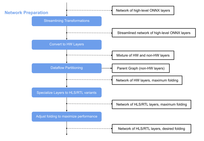
Network Preparation
The main principle of FINN are analysis and transformation passes. If you like to have more information about these please have a look at section Analysis Pass and Transformation Pass or at chapter Tutorials about the provided Jupyter notebooks.
This page is about the network preparation, the flow step that comes after the Brevitas Export. Its main idea is to optimize the network and convert the nodes to custom nodes that correspond to finn-hlslib functions. In this way we get a network that we can bring to hardware with the help of Vitis and Vivado. For that we have to apply several transformations on the ONNX model, which this flow step receives wrapped in the ModelWrapper.
Various transformations are involved in the network preparation. The following is a short overview of these.
Tidy-up transformations
These transformations do not appear in the diagram above, but are applied in many steps in the FINN flow to postprocess the model after a transformation and/or prepare it for the next transformation. They ensure that all information is set and behave like a “tidy-up”. These transformations are located in the QONNX repository and can be imported:
Streamlining Transformations
The idea behind streamlining is to eliminate floating point operations in a model by moving them around, collapsing them into one operation and transforming them into multithresholding nodes. Several transformations are involved in this step. For details have a look at the module finn.transformation.streamline and for more information on the theoretical background of this, see this paper.
After this transformation the ONNX model is streamlined and contains now custom nodes in addition to the standard nodes. At this point we can use the Functional Verification to simulate the model using Python and in the next step some of the nodes can be converted into HLS layers that correspond to finn_hlslib functions.
Convert to HW Layers
In this step standard or custom layers are converted to HW layers. HW abstraction layers are abstract (placeholder) layers that can be either implemented in HLS or as an RTL module using FINN. These layers are abstraction layers that do not directly correspond to an HLS or Verilog implementation but they will be converted in either one later in the flow.
The result is a model consisting of a mixture of HW and non-HW layers. For more details, see finn.transformation.fpgadataflow.convert_to_hw_layers.
Dataflow Partitioning
In the next step the graph is split and the part consisting of HW layers is further processed in the FINN flow. The parent graph containing the non-HW layers remains.
Specialize Layers
The network is converted to HW abstraction layers and we have excluded the non-HW layers to continue with the processing of the model. HW abstraction layers are abstract (placeholder) layers that can be either implemented in HLS or as an RTL module using FINN. In the next flow step, we convert each of these layers to either an HLS or RTL variant by calling the SpecializeLayers transformation. It is possible to let the FINN flow know a preference for the implementation style {“hls”, “rtl”} and depending on the layer type this wish will be fulfilled or it will be set to a reasonable default.
Folding
The PE and SIMD are set to 1 by default, so the result is a network of only HLS/RTL layers with maximum folding. The HLS layers of the model can be verified using the cppsim simulation. It is a simulation using C++ and is described in more detail in chapter Functional Verification.
To adjust the folding, the values for PE and SIMD can be increased to achieve also an increase in the performance. The result can be verified using the same simulation flow as for the network with maximum folding (cppsim using C++), for details please have a look at chapter Functional Verification.
The result is a network of HLS/RTL layers with desired folding and it can be passed to Hardware Build and Deployment.